MODFLOW heads on the map

aquascope.groundwater.surface.read_modflow_heads reads a MODFLOW binary head file and places its cells on the Earth, so a model's heads can be drawn on a map, the way ModelMuse, FloPy and GMS show them. The Explorer uses it when you drop a model on the globe, and the CLI and the MCP server expose the same function.

What it reads

• Heads: the binary head file (.hds, .hed, .bhd) of MODFLOW-2005 or MODFLOW 6, single or double precision, any number of layers and time steps. A drawdown file reads the same way. Each record is a 44-byte header in single precision (52 in double: kstp, kper, pertim, totim, a 16-character text, ncol, nrow, ilay), then nrow * ncol values; the precision is told from the first header. Inactive and dry cells (|h| of 1e20 and more, or -999.99 and the like) have no head. Unstructured (DISU) files are not read.
• The grid, from one of:
• a MODFLOW 6 .dis or .disv text file (DELR and DELC as CONSTANT or INTERNAL; XORIGIN, YORIGIN, ANGROT, LENGTH_UNITS from its options),
• a MODFLOW-2005 .dis (with FloPy's georeference comment when it has one),
• a MODFLOW 6 binary grid file (.dis.grb or .disv.grb), which holds every array whatever the input used, so it is the way round OPEN/CLOSE arrays,
• or a cell size, for a regular grid.
• Where and when, when the grid does not say: a .nam with the comment FloPy writes (xul/yul or xll/yll, rotation, proj4_str or epsg, start_datetime), a MODFLOW 6 .tdis (TIME_UNITS, START_DATE_TIME), or what you type: the lower-left corner, the rotation (degrees counter-clockwise) and the CRS (an EPSG code).

Cells come back as polygons in lon/lat (projected with pyproj) and heads as an array of time x layer x cell. A DIS grid with more than 60,000 cells per layer is drawn in blocks of k x k cells (their mean head), and the result says so; a DISV grid that large is refused.

Checked against FloPy

On FloPy's own examples (CC0, examples/data/mf6-freyberg and examples/data/freyberg_multilayer_transient, read on 2026-10-11, not committed) the heads are identical to flopy.utils.HeadFile's, value for value, in single and double precision (one time step on one layer, and 1,097 time steps on three layers), and the placed corners match FloPy's StructuredGrid with the same origin and rotation. A test compares the two on synthetic files wherever FloPy is installed.

Why not FloPy itself: FloPy 3.11.0 installs with micropip in the Explorer's Pyodide 314 and reads a .hds there (checked on 2026-10-11). But import flopy imports matplotlib, so the page would download about 10 MB more (matplotlib 7.0 MB, fonttools 1.2 MB, Pillow 1.0 MB, the FloPy wheel 1.5 MB, and a few small ones) to read a file whose layout fits on a page. The reader here is plain numpy and imports on a bare install.

Use it

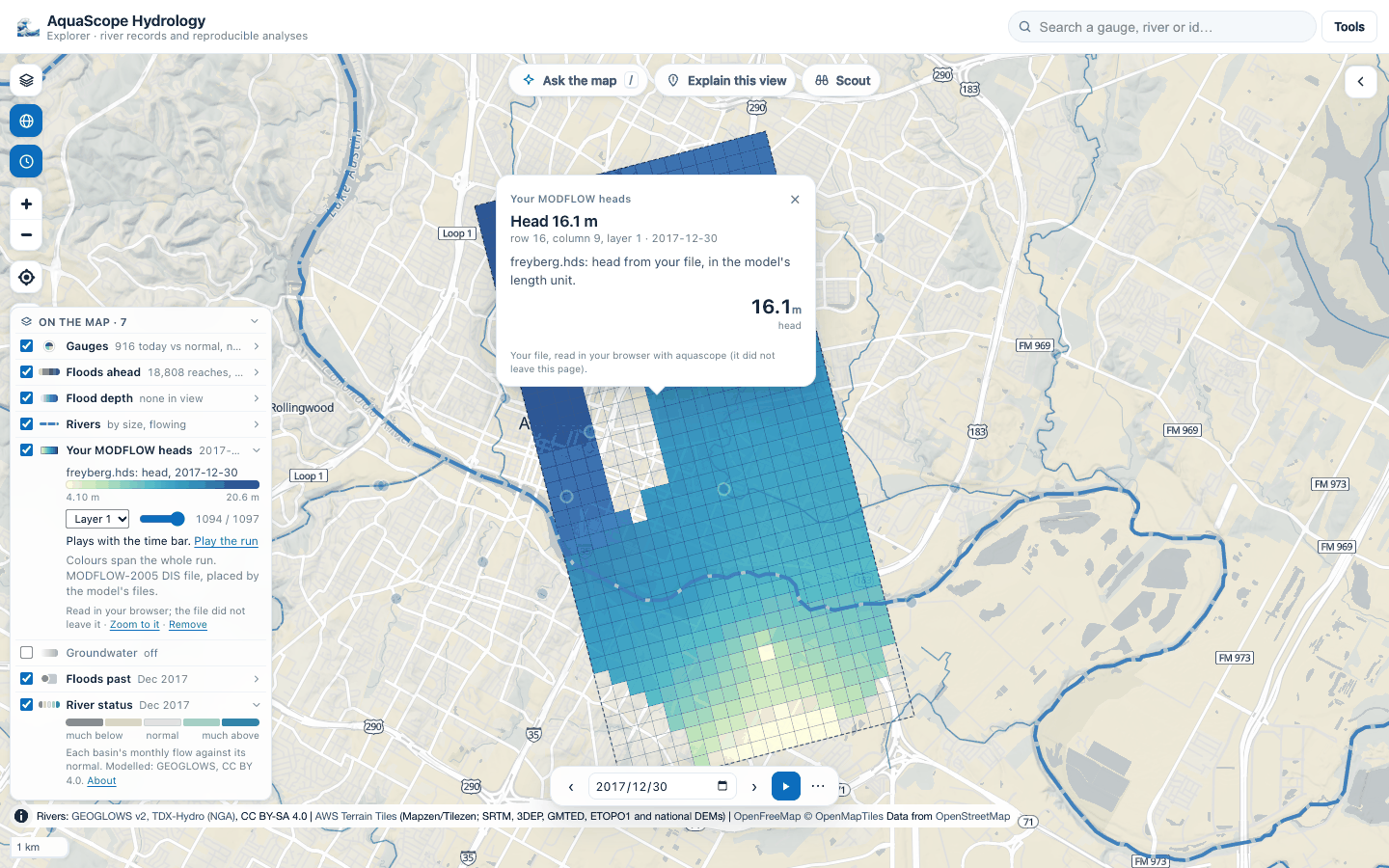
In the Explorer: drop the .hds with its grid (and the .nam if FloPy wrote one) on the map, or use Tools, Open model results, or Groundwater in the legend, then Your MODFLOW heads. The files are read in your browser's worker and do not leave it. Pick the layer, step through the times with the slider, or play the run with the time bar when the model has dates. A click on a cell gives its head. See the Explorer.

No model at hand? Tools, Open model results, MODFLOW: the Freyberg model fetches FloPy's transient Freyberg example (freyberg.nam, .dis, .hds and .wel, 11.1 MB, public domain) from FloPy's GitHub repository, pinned to one commit, and opens it like a drop. Its .nam places it; its .wel gives its six pumping wells.

A model whose files do not say where it is is never refused. The first choice is Place it at the centre of the map (approximate): one click, north up, at its true size in its own length unit (metres when the files name none). The legend row and the cell card say "approximate placement"; the heads are the model's, the place is not. The second choice is the exact form (lower-left corner, rotation, CRS), also reachable later from the legend row with Place it exactly. In Python the same is read_modflow_heads(..., approximate_at=[lon, lat]).

aquascope modflow model.hds --grid model.dis.grb --crs EPSG:27700 --origin 450000 120000
aquascope modflow freyberg.hds --grid freyberg.dis --sidecar freyberg.nam --layer 2 --geojson heads.geojson
aquascope modflow heads.hds --cell-size 100 --origin 0 0 --crs EPSG:32631 --start-date 2020-01-01

from aquascope.groundwater.surface import modflow_geojson, modflow_summary, read_modflow_heads

res = read_modflow_heads("freyberg.hds", "freyberg.dis", sidecars=["freyberg.nam"])
modflow_summary(res, time_index=-1, layer=1)    # the grid, times, dates, range and one frame, JSON-safe
modflow_geojson(res, time_index=0, layer=3)     # that frame's cells with their head

The MCP tool modflow_heads(hds_path, grid_path, ...) returns the summary and, with geojson=True, the frame's cells. When the model's place is unknown the answer says what is missing (needs: grid, origin, crs).

What it is not: a model run. It reads what MODFLOW wrote; heads are in the model's own length unit.

Contours, flow, drawdown and capture zones

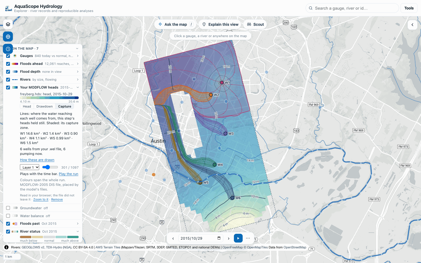
aquascope.groundwater.views (experimental, #623 and #624) reads one time step and one layer of a structured (DIS) grid the way a hydrogeologist reads a water table, and returns the geometry in lon/lat. The Explorer draws it; the CLI prints it.

• Head contours at one round interval for the whole run (so the lines hold still from step to step), heavier every fifth, drawn between cell centres (marching squares) and joined into labelled lines, over a smooth head surface.
• Flow arrows: the direction groundwater moves, down the head gradient. The gradient is a central difference between neighbouring cell centres (one-sided next to inactive cells), turned into map directions with the grid's own geometry, so a rotated grid points the right way. The direction is Darcy's law (q = -K grad h) with the same conductivity in every direction, because a head file does not hold K. The legend gives the typical direction and gradient ("mostly to the east-south-east, about 1 in 220").
• Drawdown: the head at a reference step minus the head now. The reference is the first step unless you choose another; when the wells' heads are highest at another step (a model that starts already pumping), the legend offers it, because the cone shows best measured from a step when the wells were idle.
• Wells: from a dropped .wel file (MODFLOW-2005 and NWT, or MODFLOW 6; lists in OPEN/CLOSE files are not read, and the result says so), with each stress period's rate. Without one, the cells whose drawdown is a local maximum: the drawdown used to find them is each cell's fall from its highest head in the run to its lowest, so a cone shows whether the run deepens it or lets it recover, and a candidate also has to be a head minimum at its lowest. With a single step, the local head minima. The result says which.
• Pathlines and capture zones: particles follow the head gradient within the layer (a midpoint step of a quarter cell), the step's heads held still. Forward tracking ends in a pumping well's cell; backward tracking from a ring around each well traces where its water comes from, filling in the fan where neighbouring paths drift apart, and the area those backward paths sweep is the well's capture zone, outlined, with its area. Where two wells' swept areas overlap (their paths hug the divide between them), a particle tracked forward from that spot decides which well it belongs to.

What these are not: a head file holds no hydraulic conductivity, porosity or vertical flow, so the lines are streamlines of one step in one layer, not travel times, and water that leaves the layer up or down is not followed. A well screened in another layer is shown but does not capture water in this one. For travel times and 3D paths, run MODPATH on the model.

The tests check the arrows, straight pathlines and evenly spaced straight contours on an analytic plane (a constant gradient, on a grid rotated 30 degrees too), and on the synthetic pumping well that the well is found at row 15, column 23, that the drawdown cone is centred there, and that the backward-tracked capture zone agrees with the cells whose forward paths end in the well.

aquascope modflow synthetic.hds --grid synthetic.dis --sidecar synthetic.nam --time 3 --views
aquascope modflow freyberg.hds --grid freyberg.dis --sidecar freyberg.nam --wel freyberg.wel --time 300
aquascope modflow model.hds --grid model.dis --views --reference highest --json

from aquascope.groundwater.surface import read_modflow_heads
from aquascope.groundwater.views import model_views, views_summary

res = read_modflow_heads("freyberg.hds", "freyberg.dis", sidecars=["freyberg.nam"])
v = model_views(res, time_index=300, layer=1, wells="freyberg.wel")
v["head"]["levels"]     # [{level, lines: [[[lon, lat], ...]]}]
v["flow"]["towards"]    # "south-east"
v["capture"]            # [{well, rings, area_km2, paths}]
views_summary(v)        # the same without the geometry

Layers, sections, hydrographs and the water budget

Experimental (see Stability), added after 0.27.0 for #625 and

626: aquascope.groundwater.layers and aquascope.groundwater.budget.

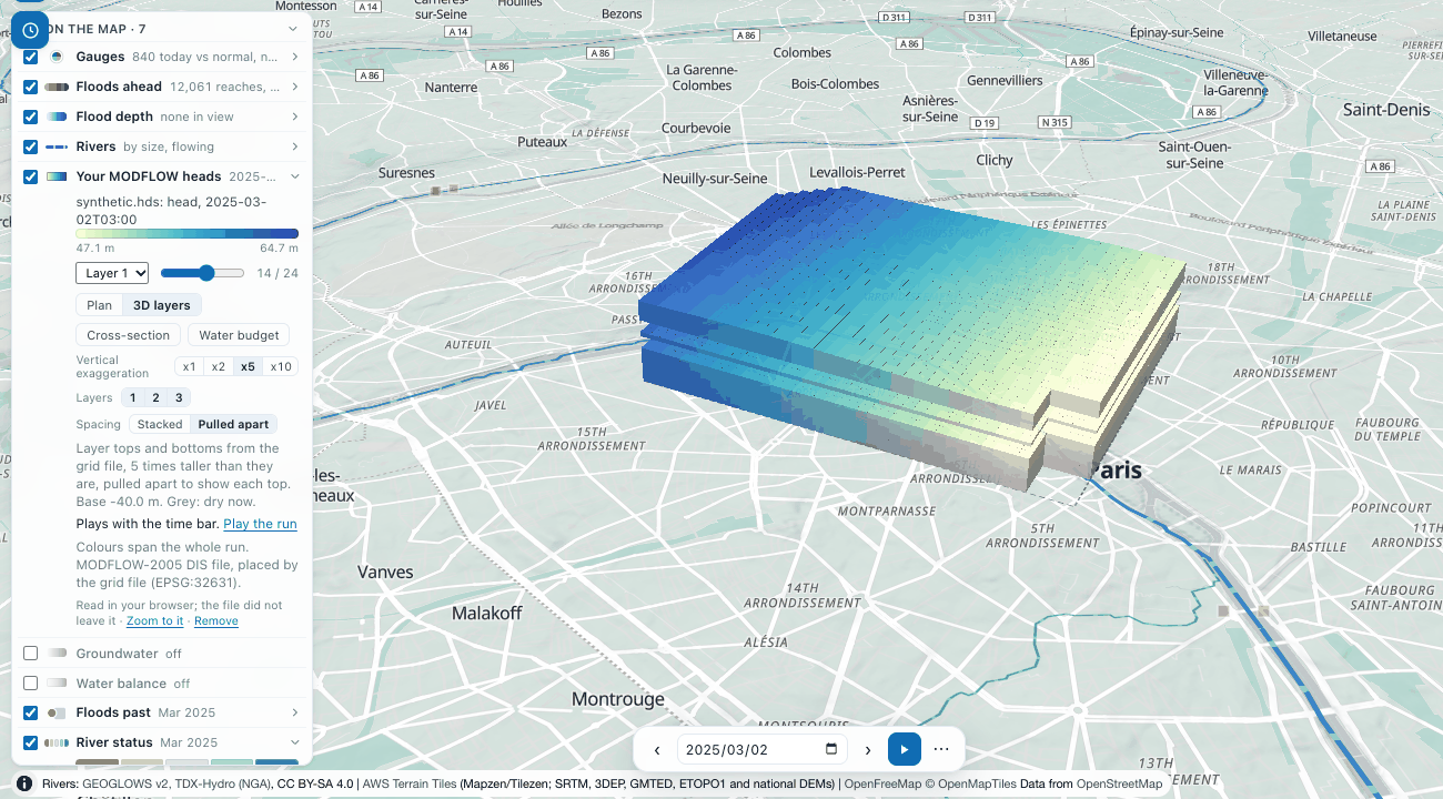
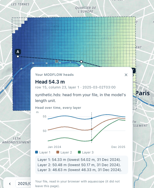
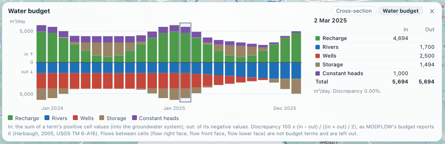
• read_layer_elevations(grid): each layer's top and bottom (TOP, BOTM, IDOMAIN) from a MODFLOW 6 .dis/.disv or .dis.grb, or a MODFLOW-2005 .dis (a confining bed under a layer, LAYCBD, is left as a gap: the next layer starts at its bottom). Checked against FloPy's ModflowDis on the Freyberg example.
• model_layers(res, grid): those elevations on the cells as read_modflow_heads draws them (block means on a big grid), the model's base and crest, and a vertical exaggeration for a 3D view: 1, 2 or 5 times a power of ten, so the stack stands about 12% of the model's width.
• cross_section(res, layers, [[lon, lat], ...]): the cells a line crosses, in order, with where it enters and leaves each (found to half a metre), every layer's top, bottom and head at every saved time, and the water table, read as the head of the uppermost layer that has one (where that head is above the layer's top, a confined layer, the notes say the line is a potentiometric surface, not a water table). Distances are on a local plane around the line (well under 1% from the geodesic over a model's few tens of kilometres).
• cell_hydrograph(res, cell, layers): one cell's head over time in every layer, with its lowest value and when, and the layer's top and bottom.
• read_budget(cbc) and water_budget(cbc, heads=res): the cell-by-cell budget file in every layout MODFLOW writes: the full layout (MODFLOW-2005 without COMPACT BUDGET), the compact one (IMETH 1 to 5) and MODFLOW 6's (IMETH 6), in single or double precision, told from the file. Per saved time and term, in is the sum of the term's positive cell values (water entering the groundwater system) and out of its negative ones; the percent discrepancy is 100 * (IN - OUT) / ((IN + OUT) / 2), as MODFLOW's own budget reports it (Harbaugh, 2005). Flows between cells (FLOW RIGHT FACE, FLOW-JA-FACE and the like) and MODFLOW 6's DATA- records are not budget terms and are left out. Rates are in the model's length cubed per its time unit. The layouts are those of the MODFLOW-2005 documentation (Harbaugh, 2005, and its Output Control input page, where COMPACT BUDGET is set) and of FloPy's CellBudgetFile; a test checks the reader against FloPy where FloPy is installed.

aquascope modflow synthetic.hds --grid synthetic.dis --sidecar synthetic.nam --time 13 \
  --layers --section 2.29,48.864 2.35,48.864 --cell 15 23 --budget synthetic.cbc

from aquascope.groundwater import budget, layers
from aquascope.groundwater.surface import read_modflow_heads

res = read_modflow_heads("synthetic.hds", "synthetic.dis", sidecars=["synthetic.nam"])
lay = layers.model_layers(res, "synthetic.dis")
sec = layers.cross_section(res, lay, [[2.29, 48.864], [2.35, 48.864]])
layers.section_summary(sec, time_index=13)       # the cells, tops, bottoms, heads and water table, JSON-safe
layers.cell_hydrograph(res, 14 * 40 + 22, lay)    # row 15, column 23: every layer's head over the run
wb = budget.water_budget("synthetic.cbc", heads=res)
budget.budget_at(wb, 13)                         # each term's in, out and net, the totals and the discrepancy

The MCP tool modflow_heads takes the same as section, cell_row/cell_col and budget_path. The synthetic three-layer model these pictures come from (a sand, a clay and a chalk with a pumping well, everything made up) is written by tests/test_groundwater/synthetic_models.py OUT_DIR.